Gradient Descent Multi Linear Regression (ML From Scratch -3)
Understanding the Mathematics Behind Gradient Descent Regression and Developing a NumPy-Only Implementation for the Algorithm
By: Gurleen Kaur
Basic Linear Regression
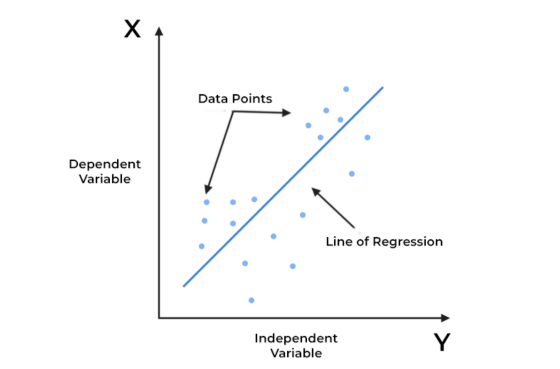
A variable’s value can be predicted using linear regression analysis based on the value of another variable. The dependent variable is the one you want to predict. The independent variable is the one you’re using to make a prediction about the value of the other variable.
With the help of one or more independent variables that can most accurately predict the value of the dependent variable, this type of analysis calculates the coefficients of the linear equation. The differences between expected and actual output values are minimised by linear regression by fitting a straight line or surface.
Linear Regression Gradient Descent
Gradient descent is an indeterministic stochastic method for minimising the error in a regression issue. As a result, we strive to obtain an approximation of the answer rather than the precise closed form solution while using this method. The least squares approach is the closed-form answer.

Math Behind Linear Regression Gradient Descent
It is a very simple approach following a 5 step procedure
- Initialize the wights and intercept to zero.
- Use current model to make prediction.
- Calculate Error(Cost) from the prediction.
- Update the weights according to the Error.
- Repeat steps 2 to 4 untill a statisfactory result is reached.
With 2 major problems that we need to keep in mind
- How to setup the Cost function(That will evaluate and represent error/loss of the current model)
- How to update the weights.
Let’s pass through them one by one
1. Cost Function:
Simply said, a cost function is a function that can estimate the inaccuracy across the entire dataset. Additionally, we are aware that a single prediction’s error is determined by:

We may now square the error to remove the negative sign and then add all of the errors for the n predictions to evaluate a cost function.

Additionally, since the total amount of errors could become extremely big, the value can be normalised by dividing it by the n samples in the dataset.

The Mean Squared Error, or MSE, is the cost function typically applied in linear regression.
2. Updating Weights
There are two key gradients that need to be kept in mind while changing the weights
- The amount of change.
- The direction of change(increase or decrease).
and both can be extracted from the gradient of the cost function.
The cost function’s slope will always go in the direction of the minimum, and its value can be used to determine how far away the minimum point actually is from the slope’s minimum point. As we move further away from the minimum, the slope rises from zero at the minimum.
So, we established that we can determine the direction and magnitude by which we need to adjust the weights by computing the Gradient of the Cost Function. The gradient’s own calculation is all that remains at this point.
Let’s first determine the gradient in relation to the weights :

Now, Calculating Gradient with respect to intercept:

Each step has been completed. One more thing, since we will be including a learning rate in the algorithm, we may omit the constant term in both equations (2 does nothing).
The gradient has now changed to:

The update rule will now be scaled with a constant learning rate(Lr). Thus, our update rule will finally change to

The entire Gradient Descent Method is now complete.
So, Lets take at the practical Implementation
Implementing The developed Gradient Descent Linear Regression
To work on the implementation part, we first need a sample dataset on which we can test our algorithm. Here, using the sklearn library, we have generated a random regression problem.
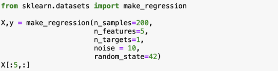
Now we extract the first five rows of our generated data to get a better understanding.

- Next, we move on to creating the gradient descent algorithm, where first we will initialize the weight vector and the intercept.
- As a part of the next step, we will set the number of iterations followed by setting the learning rate.
- Next we will calculate the gradient based off which we will update our parameters i.e. the weight and the intercept.

- Next we move on to testing our Algorithm by setting an instances and fitting our model.

- For that, we start off by checking our previously computed weight and intercept.

- We can compare the coefficients and intercept from Sklearn linear regression to evaluate the algorithm.

- We should obtain equivalent results even though Sklearn employs a least squares approach, so the coefficients won’t be exactly the same.

- As anticipated, the model is quite similar, hence we can use it as validation for our algorithm
- Now let us check the same for the predicted value of 10 randomly selected entries by making a dataframe of the actual and the predicted results.
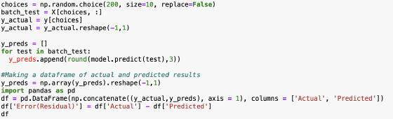

- As we can observe, the results are close and comparable even though they are not exact.
Conclusion:
- This was a brief about the Gradient Descent with linear Regression model.
- In the following articles, I will likely discuss more about other Machine Learning Models and their use cases.
- Follow me for more upcoming data science, Machine Learning, and artificial intelligence articles.
Final Thoughts and Closing Comments
There are some vital points many people fail to understand while they pursue their Data Science or AI journey. If you are one of them and looking for a way to counterbalance these cons, check out the certification programs provided by INSAID on their website. If you liked this story, I recommend you to go with the Global Certificate in Data Science & AI because this one will cover your foundations, machine learning algorithms, and deep neural networks (basic to advance).

